9 Regression
9.1 Evaluation of regression models
Mean squared error
This measure shows the deviation of the predicted value \hat{y} to the target value y. The squaring penalized large deviations and avoids respective cancellation of positive and negative errors.
MSE = 1/n \sum_i (y_i - \hat{y}_i)^2
from sklearn.metrics import mean_squared_error
mean_squared_error(y_true, y_pred)
More info: scikit-learn.org
R^2 score / coefficient of determination
This measure shows how much of the variance of the target/dependent variable y can be explained by the model/independent variable \hat{y}.
R^2 = 1 - \frac{\text{Unexplained Variance}}{\text{Total Variance}} = \frac{SS_{res}}{SS_{tot}} \\ SS_{res} = \sum_i(y_i-\hat{y}_i)^2 \\ SS_{tot} = \sum_i(y_i - \bar{y}_i)^2 where \bar{y} is the mean of the target y.
The value commonly reaches from 0 (model always predicts the mean of y) to 1 (perfect fit of model to data). It can however be negative (e.g. wrong model, heavy overfitting, …). The adjusted R^2 compensates for the size of the model (more variables), favoring simpler models. More info: wikipedia.org
from sklearn.metrics import r2_score
r2 = r2_score(y_true, y_pred)
More info: scikit-learn.org
9.2 Linear Models
Ordinary Least Squares
Linear models are of the form: y_i = x_i \beta + \epsilon_i = \beta_0 + \beta_1 x_{i(1)} + \beta_2 x_{i(2)} + \epsilon_i
- x_{i(d)} is the dimension d of point i. x_i is called regressor, independent, exogenous or explanatory variable. The regressors can be non-linear functions of the data.
- y_i is the observed value for the depependent variable for point i.
- \beta_0 is called bias or intercept (not the same as bias of a machine learning model).
- \beta_{0, 1...n} are the regression coefficients, \beta_{1,...n} are called slope. In linear models the regression coefficients need to be linear.
- \epsilon is the error term or noise.
Predicted values are denoted as \hat{\beta}, \hat{y}. We try to minimize the \epsilon-term using the least squared error method.
from sklearn.linear_model import LinearRegression
model = LinearRegression(fit_intercept=True)
model.fit(X, y)
More info: scikit-learn.org
Pros:
Easy to interpret
Fast to train and predict
Cons:
Assumption of linear relation between dependent and independet variables. (-> possibly underfitting)
Sensitive to outliers (-> possibly overfitting)
When comparing the strength of different coefficients: Take the scale of the feature into consideration (e.g. don’t compare “m/s” and “km/h”).
Only when the features have been standardized / normalized, you can safely compare them.
Check for robustness of coefficients: Make cross validation and obsever their variability. High variability can be a sign of correlation with other features.
Correlation does not mean causation.
r emo::ji("point_up_2")r emo::ji("nerd")
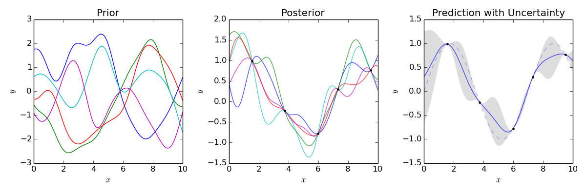
9.3 Gaussian process regression
Gaussian process regression is based on Bayesian Probability: You generate many models and calculate the probability of your models given the samples. You make predictions based on the probabilities of your models.
You get non-linear functions to your data by using non-linear kernels: You assume that input data points that are similar, will have similar target values. The concept of similarity (e.g. same hour of the day) is encoded in the kernels that you use.
Pros:
The model reports the predictions with a certain probability.
Hyperparameter tuning is built into the model.
Cons:
Training scales with O(n^3). (approximations are FITC and VFE)
You need to design or choose a kernel.
from sklearn.gaussian_process import GaussianProcessRegressor
from sklearn.gaussian_process.kernels import DotProduct, WhiteKernel, RBF, ExpSineSquared
kernel = DotProduct() + WhiteKernel() + RBF() + ExpSineSquared() # The kernel hyperparameters are tuned by the model
gpr = GaussianProcessRegressor(kernel=kernel)
gpr.fit(X, y)
gpr.predict(X, return_std=True)
More info: scikit-learn.org
9.4 Gradient boosted tree regression
Apart from classification, gradient boosted trees also allow for regression. It works like gradient boosted trees for classification: You iteratively add decision tree regressors that minimize the regression loss of the already fitted ensemble. A decision tree regressor is a decision tree that is trained on continuous data instead of discrete classification data, but its output is still discrete.
from sklearn.ensemble import GradientBoostingRegressor
gbr = GradientBoostingRegressor(n_estimators = 500, min_samples_split =5, max_depth = 4, max_features="sqrt", n_iter_no_change=15)
gbr.fit(X, y)
More info: scikit-learn.org
10 Time Series Forecasting
For “normal” settings the order of the samples does not play a role (e.g. blood sugar level of one sample is independent of the others). In time series however, the samples need to be represented in an ordered vector or matrix (e.g. The temperature of Jan 2nd is not independent of the temperature on Jan 1st).
import pandas as pd
df = pd.read_csv("data.csv", header=0, index_col=0, names=["date", "sales"])
sales_series = df["sales"] # pandas series make working with time series easier
ARIMA(X) Model
univariate time series model with exogenous regressor.
VARIMA(X) Model
Multivariate time series model, where the variables can influence each other and the target can influence the variables and vice versa.